지리 시각화 (Geospatial Visualization)

중급

학습 목표

이 레시피를 완료하면 다음을 할 수 있습니다:

위도/경도 데이터를 활용한 산점도 지도 그리기
GeoPandas를 활용한 지리 데이터 시각화

0. 사전 준비 (Setup)


import pandas as pd
import numpy as np
import matplotlib.pyplot as plt
import seaborn as sns
 
# 가상의 위치 데이터 생성 (서울 인근)
np.random.seed(42)
n_samples = 100
df_geo = pd.DataFrame({
    'lat': np.random.uniform(37.4, 37.7, n_samples),
    'lon': np.random.uniform(126.8, 127.2, n_samples),
    'value': np.random.randint(10, 100, n_samples),
    'category': np.random.choice(['A', 'B', 'C'], n_samples)
})

1. 간단한 위도/경도 산점도

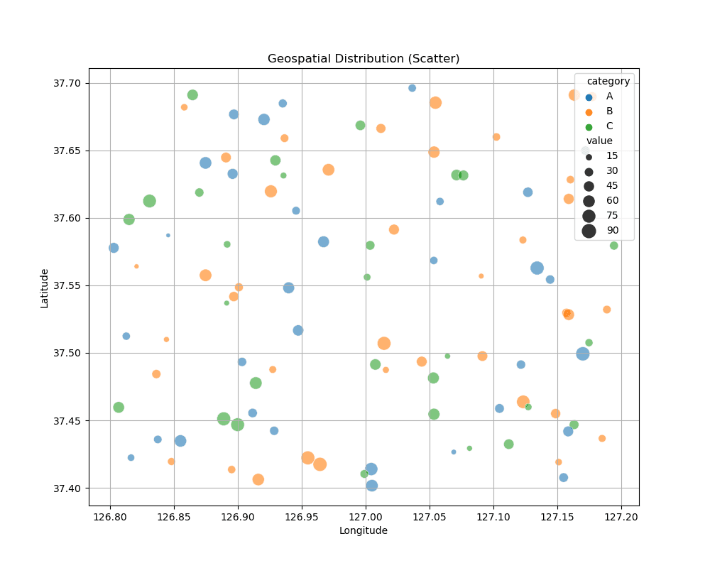
지도 파일 없이도 위도(Latitude)와 경도(Longitude)를 X, Y축으로 사용하여 대략적인 분포를 볼 수 있습니다.


plt.figure(figsize=(10, 8))
sns.scatterplot(x='lon', y='lat', hue='category', size='value', sizes=(20, 200), data=df_geo, alpha=0.6)
plt.title('Geospatial Distribution (Scatter)')
plt.xlabel('Longitude')
plt.ylabel('Latitude')
plt.grid(True)
plt.show()

실행 결과

[Graph Saved: generated_plot_fc032103bc_0.png]

Graph

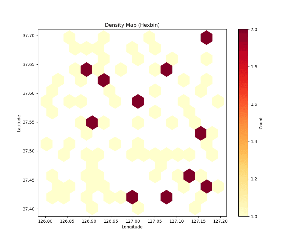
2. 헥스빈 지도 (Hexbin Map)

데이터가 많을 때 밀도를 표현하기 좋습니다.


plt.figure(figsize=(10, 8))
plt.hexbin(df_geo['lon'], df_geo['lat'], gridsize=15, cmap='YlOrRd', mincnt=1)
plt.colorbar(label='Count')
plt.title('Density Map (Hexbin)')
plt.xlabel('Longitude')
plt.ylabel('Latitude')
plt.show()

실행 결과

[Graph Saved: generated_plot_778a70b837_0.png]

Graph

3. Real Map Visualization with GeoPandas

Using geopandas, we can visualize data on actual map boundaries (World Map).


import geopandas as gpd
import matplotlib.pyplot as plt
 
# Load built-in world map dataset
# Note: 'naturalearth_lowres' download or local file required
world = gpd.read_file('src_world_map.zip')
 
# Create sample data (Capitals of some countries)
data = {
    'City': ['Seoul', 'Tokyo', 'New York', 'London', 'Sydney', 'Sao Paulo'],
    'Lat': [37.5665, 35.6762, 40.7128, 51.5074, -33.8688, -23.5505],
    'Lon': [126.9780, 139.6503, -74.0060, -0.1278, 151.2093, -46.6333],
    'Value': [100, 85, 95, 90, 80, 70]
}
df_cities = pd.DataFrame(data)
 
# Convert to GeoDataFrame
ghub_points = gpd.GeoDataFrame(
    df_cities,
    geometry=gpd.points_from_xy(df_cities.Lon, df_cities.Lat)
)
 
# Plot
fig, ax = plt.subplots(figsize=(15, 10))
 
# 1. Base Map
world.plot(ax=ax, color='lightgrey', edgecolor='white')
 
# 2. Data Points
ghub_points.plot(
    ax=ax,
    color='red',
    marker='o',
    markersize=pd.to_numeric(df_cities['Value']) * 2, # Scale size
    alpha=0.7,
    label='Major Cities'
)
 
# Labels
for x, y, label in zip(df_cities.Lon, df_cities.Lat, df_cities.City):
    ax.text(x+2, y, label, fontsize=10, fontweight='bold', color='black')
 
plt.title('Global Distribution Map (GeoPandas)', fontsize=16, fontweight='bold')
plt.xlabel('Longitude')
plt.ylabel('Latitude')
plt.legend()
plt.show()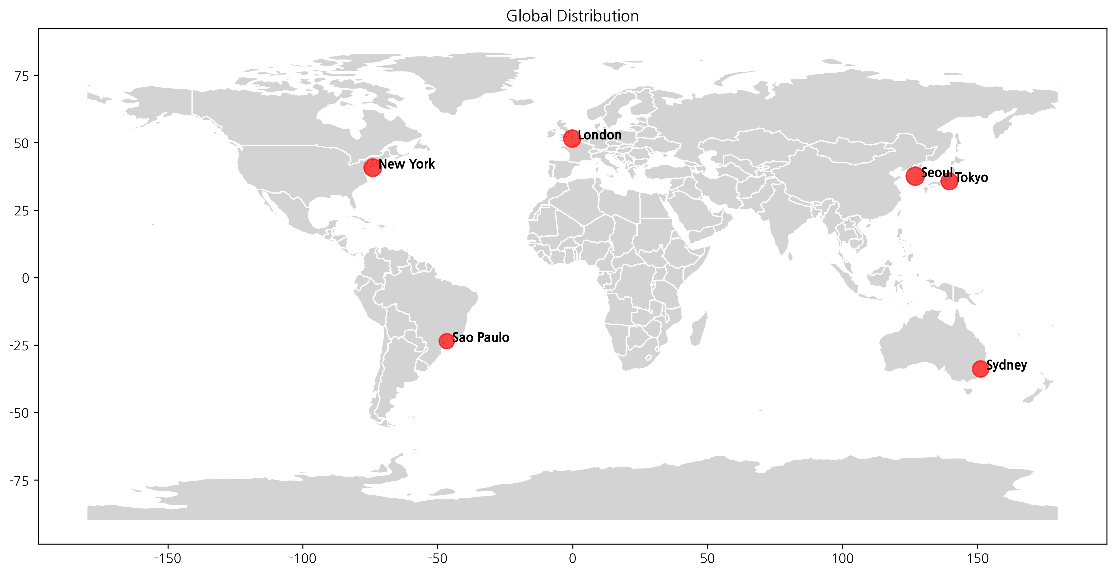

Global Distribution Map

ℹ️

The map above visualizes the distribution of major hubs using GeoPandas.