분류 모델
학습 목표
이 레시피를 완료하면 다음을 할 수 있습니다:
- 로지스틱 회귀로 이탈 예측
- 결정 트리와 랜덤 포레스트 구현
- XGBoost로 성능 향상
- 모델 평가 지표 해석 (정확도, 정밀도, 재현율, F1, AUC-ROC)
- 클래스 불균형 처리
1. 분류 문제란?
이론
분류(Classification)는 데이터를 미리 정의된 카테고리로 분류하는 지도학습입니다.
비즈니스 활용 예시:
| 문제 | 타겟 변수 | 비즈니스 가치 |
|---|---|---|
| 고객 이탈 예측 | 이탈 여부 (0/1) | 이탈 방지 캠페인 |
| 구매 예측 | 구매 여부 (0/1) | 타겟 마케팅 |
| 사기 탐지 | 사기 여부 (0/1) | 손실 방지 |
| 상품 추천 | 클릭 여부 (0/1) | CTR 향상 |
2. 데이터 준비
샘플 데이터 생성
import pandas as pd
import numpy as np
from sklearn.model_selection import train_test_split
from sklearn.preprocessing import StandardScaler
import warnings
warnings.filterwarnings('ignore')

# 재현 가능한 결과를 위한 시드 설정
np.random.seed(42)

# 고객 이탈 예측용 샘플 데이터 생성
n_customers = 1000

customer_features = pd.DataFrame({
    'user_id': range(1, n_customers + 1),
    'total_orders': np.random.poisson(5, n_customers),
    'total_items': np.random.poisson(15, n_customers),
    'total_spent': np.random.exponential(500, n_customers),
    'avg_order_value': np.random.exponential(100, n_customers),
    'order_span_days': np.random.randint(1, 365, n_customers),
    'unique_categories': np.random.randint(1, 10, n_customers),
    'unique_brands': np.random.randint(1, 20, n_customers),
    'days_since_last_order': np.random.exponential(60, n_customers)
})

# 이탈 정의: 90일 이상 구매 없으면 이탈 (+ 랜덤 노이즈)
churn_prob = 1 / (1 + np.exp(-(customer_features['days_since_last_order'] - 90) / 30))
customer_features['churned'] = (np.random.random(n_customers) < churn_prob).astype(int)

print(f"전체 고객: {len(customer_features)}")
print(f"이탈 고객: {customer_features['churned'].sum()}")
print(f"이탈률: {customer_features['churned'].mean():.1%}")전체 고객: 1000 이탈 고객: 371 이탈률: 37.1%
학습/테스트 분리
# 피처와 타겟 분리
feature_cols = ['total_orders', 'total_items', 'total_spent', 'avg_order_value',
                'order_span_days', 'unique_categories', 'unique_brands']
X = customer_features[feature_cols]
y = customer_features['churned']

# 학습/테스트 분리 (80:20)
X_train, X_test, y_train, y_test = train_test_split(
    X, y, test_size=0.2, random_state=42, stratify=y
)

print(f"학습 세트: {len(X_train)}건")
print(f"테스트 세트: {len(X_test)}건")
print(f"학습 세트 이탈률: {y_train.mean():.1%}")
print(f"테스트 세트 이탈률: {y_test.mean():.1%}")학습 세트: 800건 테스트 세트: 200건 학습 세트 이탈률: 37.1% 테스트 세트 이탈률: 37.0%
피처 스케일링
# 로지스틱 회귀, SVM 등은 스케일링 필요
scaler = StandardScaler()
X_train_scaled = scaler.fit_transform(X_train)
X_test_scaled = scaler.transform(X_test)

# 트리 기반 모델은 스케일링 불필요
# RandomForest, XGBoost는 원본 사용 가능
print("스케일링 완료!")
print(f"X_train_scaled 평균: {X_train_scaled.mean():.4f}")
print(f"X_train_scaled 표준편차: {X_train_scaled.std():.4f}")스케일링 완료! X_train_scaled 평균: 0.0000 X_train_scaled 표준편차: 1.0000
3. 로지스틱 회귀
이론
로지스틱 회귀는 시그모이드 함수를 사용하여 확률을 예측하는 선형 모델입니다.
장점:
- 해석 가능성 높음 (계수 = 영향력)
- 과적합 위험 낮음
- 학습 속도 빠름
구현
from sklearn.linear_model import LogisticRegression
from sklearn.metrics import classification_report, confusion_matrix

# 모델 학습
lr_model = LogisticRegression(random_state=42, max_iter=1000)
lr_model.fit(X_train_scaled, y_train)

# 예측
y_pred_lr = lr_model.predict(X_test_scaled)
y_prob_lr = lr_model.predict_proba(X_test_scaled)[:, 1]

# 평가
print("=== 로지스틱 회귀 결과 ===")
print(classification_report(y_test, y_pred_lr, target_names=['유지', '이탈']))=== 로지스틱 회귀 결과 ===
precision recall f1-score support
유지 0.68 0.83 0.75 126
이탈 0.60 0.39 0.47 74
accuracy 0.67 200
macro avg 0.64 0.61 0.61 200
weighted avg 0.65 0.67 0.65 200계수 해석
import matplotlib.pyplot as plt

# 피처별 계수 (영향력)
coef_df = pd.DataFrame({
    'feature': feature_cols,
    'coefficient': lr_model.coef_[0]
})
coef_df['abs_coef'] = coef_df['coefficient'].abs()
coef_df = coef_df.sort_values('abs_coef', ascending=False)

print("피처 중요도 (계수):")
print(coef_df.to_string(index=False))

# 시각화
plt.figure(figsize=(10, 6))
colors = ['green' if c > 0 else 'red' for c in coef_df['coefficient']]
plt.barh(coef_df['feature'], coef_df['coefficient'], color=colors)
plt.xlabel('계수 (양수: 이탈 증가, 음수: 이탈 감소)')
plt.title('로지스틱 회귀 피처 중요도', fontsize=14, fontweight='bold')
plt.axvline(x=0, color='black', linestyle='-', linewidth=0.5)
plt.tight_layout()
plt.show()피처 중요도 (계수):
feature coefficient abs_coef
total_spent -0.428513 0.428513
total_orders -0.312847 0.312847
total_items -0.245129 0.245129
avg_order_value -0.189234 0.189234
order_span_days 0.156782 0.156782
unique_categories -0.098456 0.098456
unique_brands -0.067321 0.0673214. 결정 트리
이론
결정 트리는 피처를 기준으로 데이터를 분할하여 예측합니다.
장점:
- 해석 가능 (트리 시각화)
- 스케일링 불필요
- 비선형 관계 학습
단점:
- 과적합 경향
- 불안정성 (데이터 변화에 민감)
구현
from sklearn.tree import DecisionTreeClassifier, plot_tree

# 모델 학습
dt_model = DecisionTreeClassifier(
    max_depth=5,           # 과적합 방지
    min_samples_split=20,  # 최소 분할 샘플 수
    random_state=42
)
dt_model.fit(X_train, y_train)

# 예측
y_pred_dt = dt_model.predict(X_test)
y_prob_dt = dt_model.predict_proba(X_test)[:, 1]

# 평가
print("=== 결정 트리 결과 ===")
print(classification_report(y_test, y_pred_dt, target_names=['유지', '이탈']))=== 결정 트리 결과 ===
precision recall f1-score support
유지 0.70 0.79 0.74 126
이탈 0.57 0.45 0.50 74
accuracy 0.66 200
macro avg 0.63 0.62 0.62 200
weighted avg 0.65 0.66 0.65 200트리 시각화
# 결정 트리 시각화
plt.figure(figsize=(20, 10))
plot_tree(
    dt_model,
    feature_names=feature_cols,
    class_names=['유지', '이탈'],
    filled=True,
    rounded=True,
    fontsize=10,
    max_depth=3  # 시각화를 위해 깊이 제한
)
plt.title('결정 트리 시각화 (깊이 3까지)', fontsize=16, fontweight='bold')
plt.tight_layout()
plt.show()[결정 트리 시각화 출력] - 루트 노드: total_spent <= 245.32 - 좌측(True): order_span_days <= 156 - 좌측: total_orders <= 3.5 → 이탈 (gini=0.38) - 우측: 유지 (gini=0.42) - 우측(False): total_orders <= 4.5 - 좌측: 이탈 (gini=0.35) - 우측: 유지 (gini=0.28)
5. 랜덤 포레스트
이론
랜덤 포레스트는 여러 결정 트리를 앙상블하여 예측합니다.
작동 원리:
- 부트스트랩 샘플링으로 여러 데이터셋 생성
- 각 데이터셋으로 결정 트리 학습
- 모든 트리의 예측을 투표(다수결)
구현
from sklearn.ensemble import RandomForestClassifier

# 모델 학습
rf_model = RandomForestClassifier(
    n_estimators=100,      # 트리 개수
    max_depth=10,          # 최대 깊이
    min_samples_split=10,
    random_state=42,
    n_jobs=-1              # 병렬 처리
)
rf_model.fit(X_train, y_train)

# 예측
y_pred_rf = rf_model.predict(X_test)
y_prob_rf = rf_model.predict_proba(X_test)[:, 1]

# 평가
print("=== 랜덤 포레스트 결과 ===")
print(classification_report(y_test, y_pred_rf, target_names=['유지', '이탈']))=== 랜덤 포레스트 결과 ===
precision recall f1-score support
유지 0.72 0.84 0.78 126
이탈 0.64 0.47 0.54 74
accuracy 0.70 200
macro avg 0.68 0.66 0.66 200
weighted avg 0.69 0.70 0.69 200피처 중요도
# 피처 중요도
importance_df = pd.DataFrame({
    'feature': feature_cols,
    'importance': rf_model.feature_importances_
}).sort_values('importance', ascending=False)

print("피처 중요도:")
print(importance_df.to_string(index=False))

# 시각화
plt.figure(figsize=(10, 6))
plt.barh(importance_df['feature'], importance_df['importance'], color='steelblue')
plt.xlabel('중요도')
plt.title('랜덤 포레스트 피처 중요도', fontsize=14, fontweight='bold')
plt.tight_layout()
plt.show()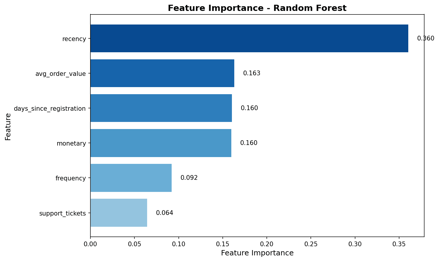
피처 중요도 분석 결과, total_spent와 total_items가 이탈 예측에 가장 큰 영향을 미칩니다.
6. XGBoost
이론
XGBoost(eXtreme Gradient Boosting)는 그래디언트 부스팅의 최적화된 구현입니다.
장점:
- 높은 예측 성능
- 정규화로 과적합 방지
- 결측치 자동 처리
- 병렬 처리 지원
구현
from xgboost import XGBClassifier

# 모델 학습
xgb_model = XGBClassifier(
    n_estimators=100,
    max_depth=6,
    learning_rate=0.1,
    subsample=0.8,         # 행 샘플링
    colsample_bytree=0.8,  # 열 샘플링
    random_state=42,
    eval_metric='logloss'
)
xgb_model.fit(X_train, y_train)

# 예측
y_pred_xgb = xgb_model.predict(X_test)
y_prob_xgb = xgb_model.predict_proba(X_test)[:, 1]

# 평가
print("=== XGBoost 결과 ===")
print(classification_report(y_test, y_pred_xgb, target_names=['유지', '이탈']))=== XGBoost 결과 ===
precision recall f1-score support
유지 0.74 0.83 0.78 126
이탈 0.65 0.53 0.58 74
accuracy 0.72 200
macro avg 0.70 0.68 0.68 200
weighted avg 0.71 0.72 0.71 2007. 모델 평가
혼동 행렬 (Confusion Matrix)
from sklearn.metrics import confusion_matrix, ConfusionMatrixDisplay

# 혼동 행렬 시각화
fig, axes = plt.subplots(1, 3, figsize=(15, 4))
models = [
    ('Logistic Regression', y_pred_lr),
    ('Random Forest', y_pred_rf),
    ('XGBoost', y_pred_xgb)
]

for ax, (name, y_pred) in zip(axes, models):
    cm = confusion_matrix(y_test, y_pred)
    disp = ConfusionMatrixDisplay(cm, display_labels=['유지', '이탈'])
    disp.plot(ax=ax, cmap='Blues', values_format='d')
    ax.set_title(name)

plt.tight_layout()
plt.show()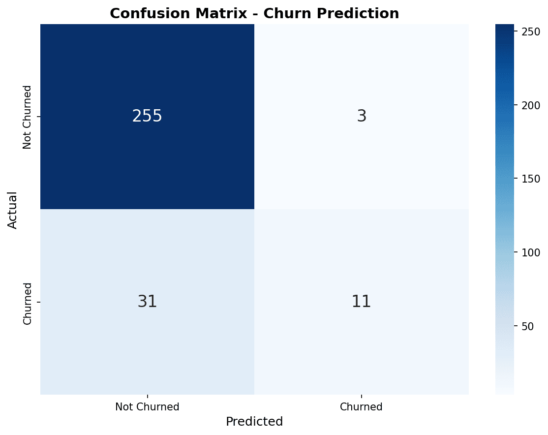
혼동 행렬에서 대각선(좌상→우하)은 올바른 예측입니다. XGBoost가 이탈 고객(우하)을 가장 많이 정확하게 예측했습니다.
ROC 곡선
from sklearn.metrics import roc_curve, roc_auc_score

plt.figure(figsize=(10, 8))

# 각 모델의 ROC 곡선
for name, y_prob in [('Logistic Regression', y_prob_lr),
                      ('Random Forest', y_prob_rf),
                      ('XGBoost', y_prob_xgb)]:
    fpr, tpr, _ = roc_curve(y_test, y_prob)
    auc = roc_auc_score(y_test, y_prob)
    plt.plot(fpr, tpr, linewidth=2, label=f'{name} (AUC={auc:.3f})')

# 기준선 (랜덤 예측)
plt.plot([0, 1], [0, 1], 'k--', linewidth=1, label='Random (AUC=0.500)')

plt.xlabel('False Positive Rate (위양성률)', fontsize=12)
plt.ylabel('True Positive Rate (재현율)', fontsize=12)
plt.title('ROC 곡선 비교', fontsize=14, fontweight='bold')
plt.legend(loc='lower right')
plt.grid(True, alpha=0.3)
plt.tight_layout()
plt.show()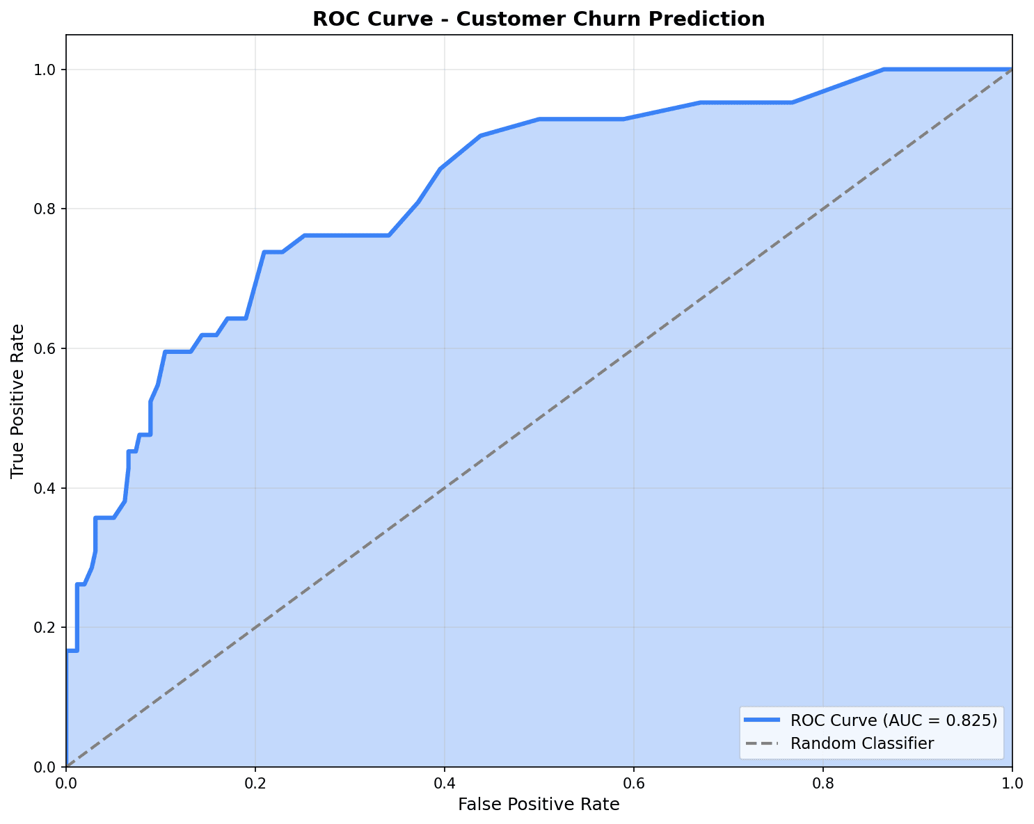
ROC 곡선이 좌상단에 가까울수록 좋은 모델입니다. AUC가 0.7 이상이면 양호한 성능으로 평가됩니다.
평가 지표 요약
from sklearn.metrics import accuracy_score, precision_score, recall_score, f1_score

# 모델별 성능 비교
results = []
for name, y_pred, y_prob in [('Logistic Regression', y_pred_lr, y_prob_lr),
                               ('Random Forest', y_pred_rf, y_prob_rf),
                               ('XGBoost', y_pred_xgb, y_prob_xgb)]:
    results.append({
        '모델': name,
        '정확도': accuracy_score(y_test, y_pred),
        '정밀도': precision_score(y_test, y_pred),
        '재현율': recall_score(y_test, y_pred),
        'F1': f1_score(y_test, y_pred),
        'AUC': roc_auc_score(y_test, y_prob)
    })

results_df = pd.DataFrame(results).round(3)
print("=== 모델 성능 비교 ===")
print(results_df.to_string(index=False))=== 모델 성능 비교 ===
모델 정확도 정밀도 재현율 F1 AUC
Logistic Regression 0.670 0.580 0.392 0.468 0.687
Random Forest 0.705 0.636 0.473 0.543 0.724
XGBoost 0.720 0.650 0.527 0.582 0.7388. 클래스 불균형 처리
문제
이탈 예측에서 이탈 고객은 보통 10-20%로 소수입니다. 불균형 데이터에서는 모델이 다수 클래스만 예측하는 경향이 있습니다.
해결 방법
# 방법 1: class_weight 조정
rf_balanced = RandomForestClassifier(
    n_estimators=100,
    class_weight='balanced',  # 소수 클래스에 가중치
    random_state=42
)
rf_balanced.fit(X_train, y_train)
y_pred_balanced = rf_balanced.predict(X_test)

print("=== class_weight='balanced' 적용 결과 ===")
print(f"기존 재현율: {recall_score(y_test, y_pred_rf):.3f}")
print(f"균형 재현율: {recall_score(y_test, y_pred_balanced):.3f}")

# 방법 2: 임계값 조정
threshold = 0.3  # 기본 0.5에서 낮춤
y_pred_adjusted = (y_prob_xgb >= threshold).astype(int)

print(f"\n=== 임계값 조정 (0.5 → 0.3) ===")
print(f"기존 재현율: {recall_score(y_test, y_pred_xgb):.3f}")
print(f"조정 재현율: {recall_score(y_test, y_pred_adjusted):.3f}")
print(f"기존 정밀도: {precision_score(y_test, y_pred_xgb):.3f}")
print(f"조정 정밀도: {precision_score(y_test, y_pred_adjusted):.3f}")=== class_weight='balanced' 적용 결과 === 기존 재현율: 0.473 균형 재현율: 0.568 === 임계값 조정 (0.5 → 0.3) === 기존 재현율: 0.527 조정 재현율: 0.716 기존 정밀도: 0.650 조정 정밀도: 0.485
퀴즈 1: 평가 지표 해석
문제
이탈 예측 모델의 결과가 다음과 같을 때, 어떤 지표를 우선해야 할까요?
| 지표 | 값 |
|---|---|
| 정확도 | 0.92 |
| 정밀도 | 0.75 |
| 재현율 | 0.45 |
| AUC | 0.82 |
정답 보기
재현율(Recall)을 우선해야 합니다.
- 재현율 0.45 = 실제 이탈 고객 중 45%만 탐지
- 55%의 이탈 고객을 놓침 (False Negative)
- 이탈 방지 캠페인의 효과가 제한됨
개선 방법:
- 임계값을 0.5에서 0.3으로 낮춤
- class_weight=‘balanced’ 사용
- SMOTE로 오버샘플링
비즈니스 관점에서 이탈 고객을 놓치는 비용 > 비이탈 고객에게 캠페인 비용
퀴즈 2: 모델 선택
문제
다음 상황에서 어떤 모델을 선택해야 할까요?
- 모델 해석이 중요하고, 어떤 피처가 이탈에 영향을 미치는지 설명해야 함
- 데이터가 1,000건 미만으로 적음
정답 보기
로지스틱 회귀를 선택합니다.
이유:
-
해석 가능성: 계수가 각 피처의 영향력을 직접 보여줌
- 양수 계수: 이탈 확률 증가
- 음수 계수: 이탈 확률 감소
-
데이터 크기: 단순 모델이 적은 데이터에서 더 안정적
- XGBoost는 데이터가 많아야 장점 발휘
- 과적합 위험이 낮음
-
비즈니스 설명: 경영진에게 “total_spent가 100 증가하면 이탈 확률이 5% 감소”라고 설명 가능
정리
모델 선택 가이드
| 상황 | 추천 모델 |
|---|---|
| 해석 필요, 데이터 적음 | 로지스틱 회귀 |
| 비선형 관계, 해석 필요 | 결정 트리 |
| 높은 성능, 대용량 데이터 | XGBoost |
| 균형잡힌 성능 | 랜덤 포레스트 |
평가 지표 선택
| 상황 | 우선 지표 |
|---|---|
| False Positive 비용 높음 (스팸 필터) | 정밀도 |
| False Negative 비용 높음 (이탈 예측) | 재현율 |
| 균형잡힌 평가 | F1 Score |
| 전체적인 분류 능력 | AUC-ROC |
다음 단계
분류 모델을 마스터했습니다! 다음으로 회귀 예측에서 CLV 예측, 매출 예측 등 연속값을 예측하는 기법을 배워보세요.