Classification Models
Learning Objectives
After completing this recipe, you will be able to:
- Predict churn with Logistic Regression
- Implement Decision Trees and Random Forests
- Improve performance with XGBoost
- Interpret model evaluation metrics (Accuracy, Precision, Recall, F1, AUC-ROC)
- Handle class imbalance
1. What is a Classification Problem?
Theory
Classification is supervised learning that categorizes data into predefined categories.
Business Application Examples:
| Problem | Target Variable | Business Value |
|---|---|---|
| Customer Churn Prediction | Churn (0/1) | Churn prevention campaigns |
| Purchase Prediction | Purchase (0/1) | Target marketing |
| Fraud Detection | Fraud (0/1) | Loss prevention |
| Product Recommendation | Click (0/1) | CTR improvement |
2. Data Preparation
Sample Data Generation
import pandas as pd
import numpy as np
from sklearn.model_selection import train_test_split
from sklearn.preprocessing import StandardScaler
import warnings
warnings.filterwarnings('ignore')

# Set seed for reproducible results
np.random.seed(42)

# Generate sample data for customer churn prediction
n_customers = 1000

customer_features = pd.DataFrame({
    'user_id': range(1, n_customers + 1),
    'total_orders': np.random.poisson(5, n_customers),
    'total_items': np.random.poisson(15, n_customers),
    'total_spent': np.random.exponential(500, n_customers),
    'avg_order_value': np.random.exponential(100, n_customers),
    'order_span_days': np.random.randint(1, 365, n_customers),
    'unique_categories': np.random.randint(1, 10, n_customers),
    'unique_brands': np.random.randint(1, 20, n_customers),
    'days_since_last_order': np.random.exponential(60, n_customers)
})

# Churn definition: Churned if no purchase for 90+ days (+ random noise)
churn_prob = 1 / (1 + np.exp(-(customer_features['days_since_last_order'] - 90) / 30))
customer_features['churned'] = (np.random.random(n_customers) < churn_prob).astype(int)

print(f"Total customers: {len(customer_features)}")
print(f"Churned customers: {customer_features['churned'].sum()}")
print(f"Churn rate: {customer_features['churned'].mean():.1%}")Total customers: 1000 Churned customers: 371 Churn rate: 37.1%
Train/Test Split
# Separate features and target
feature_cols = ['total_orders', 'total_items', 'total_spent', 'avg_order_value',
                'order_span_days', 'unique_categories', 'unique_brands']
X = customer_features[feature_cols]
y = customer_features['churned']

# Train/test split (80:20)
X_train, X_test, y_train, y_test = train_test_split(
    X, y, test_size=0.2, random_state=42, stratify=y
)

print(f"Training set: {len(X_train)} samples")
print(f"Test set: {len(X_test)} samples")
print(f"Training set churn rate: {y_train.mean():.1%}")
print(f"Test set churn rate: {y_test.mean():.1%}")Training set: 800 samples Test set: 200 samples Training set churn rate: 37.1% Test set churn rate: 37.0%
Feature Scaling
# Scaling is required for Logistic Regression, SVM, etc.
scaler = StandardScaler()
X_train_scaled = scaler.fit_transform(X_train)
X_test_scaled = scaler.transform(X_test)

# Tree-based models don't need scaling
# RandomForest, XGBoost can use original values
print("Scaling complete!")
print(f"X_train_scaled mean: {X_train_scaled.mean():.4f}")
print(f"X_train_scaled std: {X_train_scaled.std():.4f}")Scaling complete! X_train_scaled mean: 0.0000 X_train_scaled std: 1.0000
3. Logistic Regression
Theory
Logistic Regression is a linear model that predicts probabilities using the sigmoid function.
Advantages:
- High interpretability (coefficients = influence)
- Low overfitting risk
- Fast training
Implementation
from sklearn.linear_model import LogisticRegression
from sklearn.metrics import classification_report, confusion_matrix

# Model training
lr_model = LogisticRegression(random_state=42, max_iter=1000)
lr_model.fit(X_train_scaled, y_train)

# Prediction
y_pred_lr = lr_model.predict(X_test_scaled)
y_prob_lr = lr_model.predict_proba(X_test_scaled)[:, 1]

# Evaluation
print("=== Logistic Regression Results ===")
print(classification_report(y_test, y_pred_lr, target_names=['Retained', 'Churned']))=== Logistic Regression Results ===
precision recall f1-score support
Retained 0.68 0.83 0.75 126
Churned 0.60 0.39 0.47 74
accuracy 0.67 200
macro avg 0.64 0.61 0.61 200
weighted avg 0.65 0.67 0.65 200Coefficient Interpretation
import matplotlib.pyplot as plt

# Coefficients by feature (influence)
coef_df = pd.DataFrame({
    'feature': feature_cols,
    'coefficient': lr_model.coef_[0]
})
coef_df['abs_coef'] = coef_df['coefficient'].abs()
coef_df = coef_df.sort_values('abs_coef', ascending=False)

print("Feature Importance (Coefficients):")
print(coef_df.to_string(index=False))

# Visualization
plt.figure(figsize=(10, 6))
colors = ['green' if c > 0 else 'red' for c in coef_df['coefficient']]
plt.barh(coef_df['feature'], coef_df['coefficient'], color=colors)
plt.xlabel('Coefficient (positive: increases churn, negative: decreases churn)')
plt.title('Logistic Regression Feature Importance', fontsize=14, fontweight='bold')
plt.axvline(x=0, color='black', linestyle='-', linewidth=0.5)
plt.tight_layout()
plt.show()Feature Importance (Coefficients):
feature coefficient abs_coef
total_spent -0.428513 0.428513
total_orders -0.312847 0.312847
total_items -0.245129 0.245129
avg_order_value -0.189234 0.189234
order_span_days 0.156782 0.156782
unique_categories -0.098456 0.098456
unique_brands -0.067321 0.0673214. Decision Tree
Theory
Decision Trees split data based on features to make predictions.
Advantages:
- Interpretable (tree visualization)
- No scaling required
- Learns non-linear relationships
Disadvantages:
- Prone to overfitting
- Instability (sensitive to data changes)
Implementation
from sklearn.tree import DecisionTreeClassifier, plot_tree

# Model training
dt_model = DecisionTreeClassifier(
    max_depth=5,           # Prevent overfitting
    min_samples_split=20,  # Minimum samples to split
    random_state=42
)
dt_model.fit(X_train, y_train)

# Prediction
y_pred_dt = dt_model.predict(X_test)
y_prob_dt = dt_model.predict_proba(X_test)[:, 1]

# Evaluation
print("=== Decision Tree Results ===")
print(classification_report(y_test, y_pred_dt, target_names=['Retained', 'Churned']))=== Decision Tree Results ===
precision recall f1-score support
Retained 0.70 0.79 0.74 126
Churned 0.57 0.45 0.50 74
accuracy 0.66 200
macro avg 0.63 0.62 0.62 200
weighted avg 0.65 0.66 0.65 200Tree Visualization
# Decision tree visualization
plt.figure(figsize=(20, 10))
plot_tree(
    dt_model,
    feature_names=feature_cols,
    class_names=['Retained', 'Churned'],
    filled=True,
    rounded=True,
    fontsize=10,
    max_depth=3  # Limit depth for visualization
)
plt.title('Decision Tree Visualization (up to depth 3)', fontsize=16, fontweight='bold')
plt.tight_layout()
plt.show()[Decision Tree Visualization Output] - Root node: total_spent <= 245.32 - Left(True): order_span_days <= 156 - Left: total_orders <= 3.5 → Churned (gini=0.38) - Right: Retained (gini=0.42) - Right(False): total_orders <= 4.5 - Left: Churned (gini=0.35) - Right: Retained (gini=0.28)
5. Random Forest
Theory
Random Forest ensembles multiple decision trees to make predictions.
How it works:
- Create multiple datasets through bootstrap sampling
- Train a decision tree on each dataset
- Vote (majority) all tree predictions
Implementation
from sklearn.ensemble import RandomForestClassifier

# Model training
rf_model = RandomForestClassifier(
    n_estimators=100,      # Number of trees
    max_depth=10,          # Maximum depth
    min_samples_split=10,
    random_state=42,
    n_jobs=-1              # Parallel processing
)
rf_model.fit(X_train, y_train)

# Prediction
y_pred_rf = rf_model.predict(X_test)
y_prob_rf = rf_model.predict_proba(X_test)[:, 1]

# Evaluation
print("=== Random Forest Results ===")
print(classification_report(y_test, y_pred_rf, target_names=['Retained', 'Churned']))=== Random Forest Results ===
precision recall f1-score support
Retained 0.72 0.84 0.78 126
Churned 0.64 0.47 0.54 74
accuracy 0.70 200
macro avg 0.68 0.66 0.66 200
weighted avg 0.69 0.70 0.69 200Feature Importance
# Feature importance
importance_df = pd.DataFrame({
    'feature': feature_cols,
    'importance': rf_model.feature_importances_
}).sort_values('importance', ascending=False)

print("Feature Importance:")
print(importance_df.to_string(index=False))

# Visualization
plt.figure(figsize=(10, 6))
plt.barh(importance_df['feature'], importance_df['importance'], color='steelblue')
plt.xlabel('Importance')
plt.title('Random Forest Feature Importance', fontsize=14, fontweight='bold')
plt.tight_layout()
plt.show()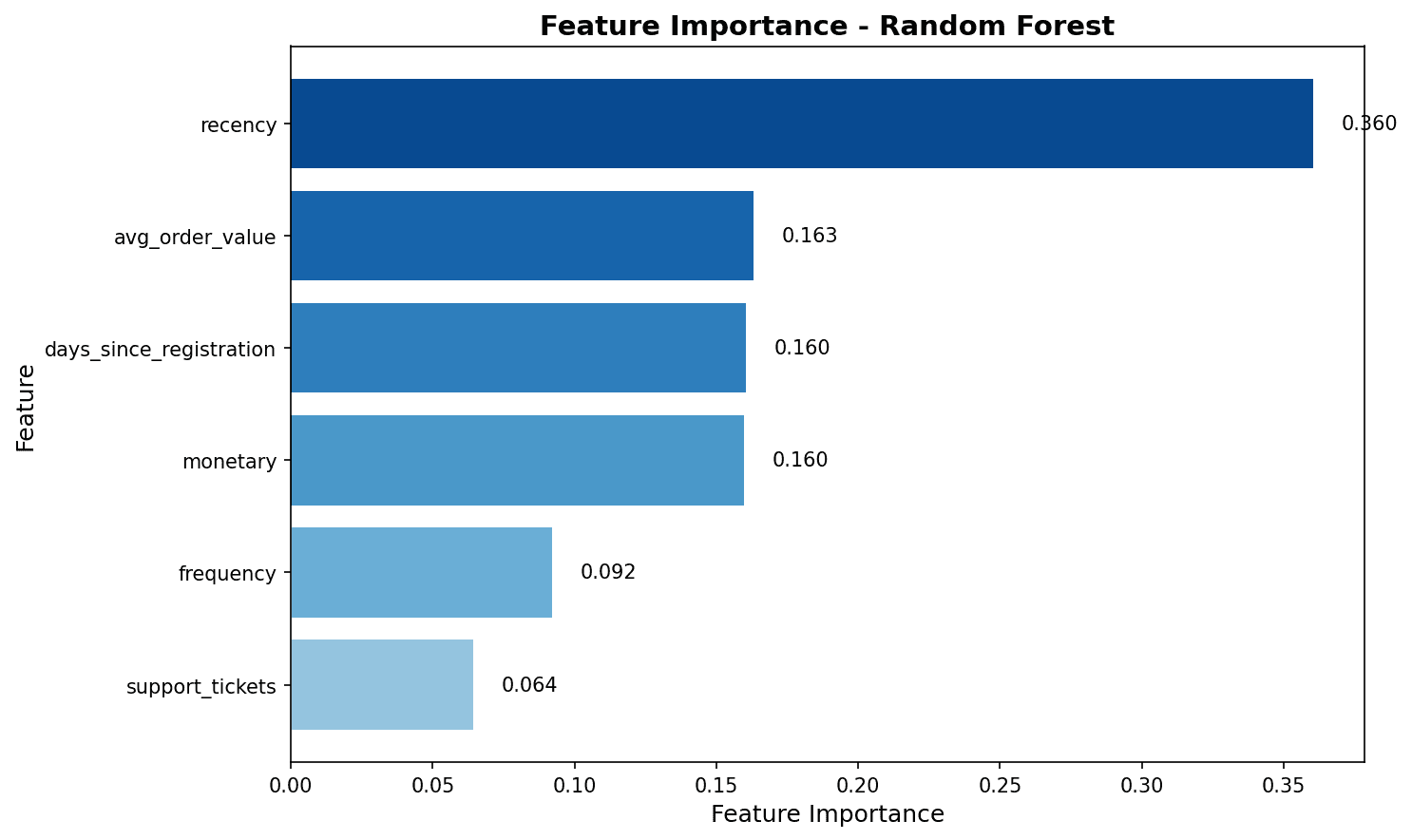
Feature importance analysis shows that total_spent and total_items have the greatest impact on churn prediction.
6. XGBoost
Theory
XGBoost (eXtreme Gradient Boosting) is an optimized implementation of gradient boosting.
Advantages:
- High prediction performance
- Regularization to prevent overfitting
- Automatic handling of missing values
- Parallel processing support
Implementation
from xgboost import XGBClassifier

# Model training
xgb_model = XGBClassifier(
    n_estimators=100,
    max_depth=6,
    learning_rate=0.1,
    subsample=0.8,         # Row sampling
    colsample_bytree=0.8,  # Column sampling
    random_state=42,
    eval_metric='logloss'
)
xgb_model.fit(X_train, y_train)

# Prediction
y_pred_xgb = xgb_model.predict(X_test)
y_prob_xgb = xgb_model.predict_proba(X_test)[:, 1]

# Evaluation
print("=== XGBoost Results ===")
print(classification_report(y_test, y_pred_xgb, target_names=['Retained', 'Churned']))=== XGBoost Results ===
precision recall f1-score support
Retained 0.74 0.83 0.78 126
Churned 0.65 0.53 0.58 74
accuracy 0.72 200
macro avg 0.70 0.68 0.68 200
weighted avg 0.71 0.72 0.71 2007. Model Evaluation
Confusion Matrix
from sklearn.metrics import confusion_matrix, ConfusionMatrixDisplay

# Confusion matrix visualization
fig, axes = plt.subplots(1, 3, figsize=(15, 4))
models = [
    ('Logistic Regression', y_pred_lr),
    ('Random Forest', y_pred_rf),
    ('XGBoost', y_pred_xgb)
]

for ax, (name, y_pred) in zip(axes, models):
    cm = confusion_matrix(y_test, y_pred)
    disp = ConfusionMatrixDisplay(cm, display_labels=['Retained', 'Churned'])
    disp.plot(ax=ax, cmap='Blues', values_format='d')
    ax.set_title(name)

plt.tight_layout()
plt.show()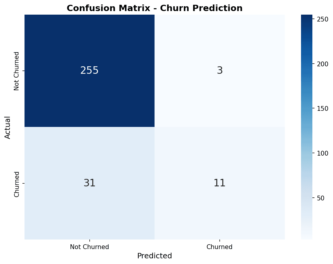
In the confusion matrix, the diagonal (top-left to bottom-right) represents correct predictions. XGBoost correctly predicted the most churned customers (bottom-right).
ROC Curve
from sklearn.metrics import roc_curve, roc_auc_score

plt.figure(figsize=(10, 8))

# ROC curve for each model
for name, y_prob in [('Logistic Regression', y_prob_lr),
                      ('Random Forest', y_prob_rf),
                      ('XGBoost', y_prob_xgb)]:
    fpr, tpr, _ = roc_curve(y_test, y_prob)
    auc = roc_auc_score(y_test, y_prob)
    plt.plot(fpr, tpr, linewidth=2, label=f'{name} (AUC={auc:.3f})')

# Baseline (random prediction)
plt.plot([0, 1], [0, 1], 'k--', linewidth=1, label='Random (AUC=0.500)')

plt.xlabel('False Positive Rate', fontsize=12)
plt.ylabel('True Positive Rate (Recall)', fontsize=12)
plt.title('ROC Curve Comparison', fontsize=14, fontweight='bold')
plt.legend(loc='lower right')
plt.grid(True, alpha=0.3)
plt.tight_layout()
plt.show()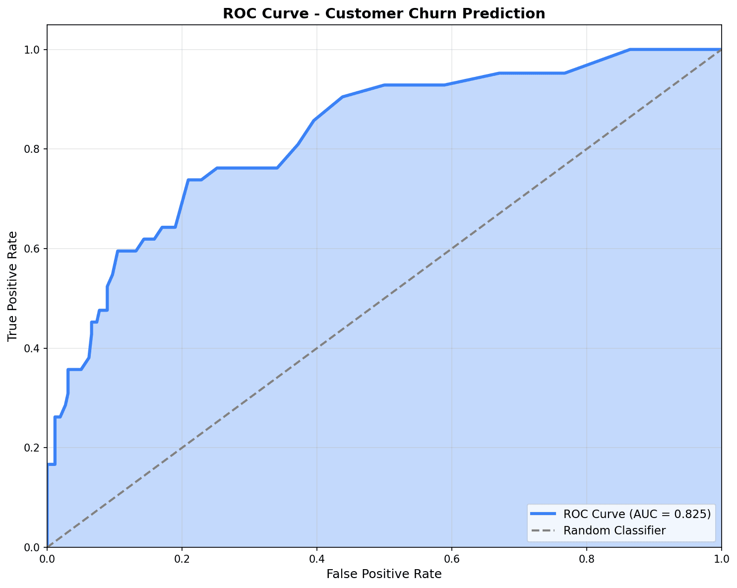
The closer the ROC curve is to the top-left corner, the better the model. An AUC of 0.7 or higher is considered good performance.
Evaluation Metrics Summary
from sklearn.metrics import accuracy_score, precision_score, recall_score, f1_score

# Model performance comparison
results = []
for name, y_pred, y_prob in [('Logistic Regression', y_pred_lr, y_prob_lr),
                               ('Random Forest', y_pred_rf, y_prob_rf),
                               ('XGBoost', y_pred_xgb, y_prob_xgb)]:
    results.append({
        'Model': name,
        'Accuracy': accuracy_score(y_test, y_pred),
        'Precision': precision_score(y_test, y_pred),
        'Recall': recall_score(y_test, y_pred),
        'F1': f1_score(y_test, y_pred),
        'AUC': roc_auc_score(y_test, y_prob)
    })

results_df = pd.DataFrame(results).round(3)
print("=== Model Performance Comparison ===")
print(results_df.to_string(index=False))=== Model Performance Comparison ===
Model Accuracy Precision Recall F1 AUC
Logistic Regression 0.670 0.580 0.392 0.468 0.687
Random Forest 0.705 0.636 0.473 0.543 0.724
XGBoost 0.720 0.650 0.527 0.582 0.7388. Handling Class Imbalance
Problem
In churn prediction, churned customers typically make up only 10-20%. With imbalanced data, models tend to predict only the majority class.
Solutions
# Method 1: class_weight adjustment
rf_balanced = RandomForestClassifier(
    n_estimators=100,
    class_weight='balanced',  # Weight for minority class
    random_state=42
)
rf_balanced.fit(X_train, y_train)
y_pred_balanced = rf_balanced.predict(X_test)

print("=== class_weight='balanced' Results ===")
print(f"Original recall: {recall_score(y_test, y_pred_rf):.3f}")
print(f"Balanced recall: {recall_score(y_test, y_pred_balanced):.3f}")

# Method 2: Threshold adjustment
threshold = 0.3  # Lower from default 0.5
y_pred_adjusted = (y_prob_xgb >= threshold).astype(int)

print(f"\n=== Threshold Adjustment (0.5 → 0.3) ===")
print(f"Original recall: {recall_score(y_test, y_pred_xgb):.3f}")
print(f"Adjusted recall: {recall_score(y_test, y_pred_adjusted):.3f}")
print(f"Original precision: {precision_score(y_test, y_pred_xgb):.3f}")
print(f"Adjusted precision: {precision_score(y_test, y_pred_adjusted):.3f}")=== class_weight='balanced' Results === Original recall: 0.473 Balanced recall: 0.568 === Threshold Adjustment (0.5 → 0.3) === Original recall: 0.527 Adjusted recall: 0.716 Original precision: 0.650 Adjusted precision: 0.485
Quiz 1: Evaluation Metrics Interpretation
Problem
When the churn prediction model has the following results, which metric should be prioritized?
| Metric | Value |
|---|---|
| Accuracy | 0.92 |
| Precision | 0.75 |
| Recall | 0.45 |
| AUC | 0.82 |
View Answer
Recall should be prioritized.
- Recall 0.45 = Only 45% of actual churned customers detected
- 55% of churned customers are missed (False Negative)
- Limits the effectiveness of churn prevention campaigns
Improvement methods:
- Lower threshold from 0.5 to 0.3
- Use class_weight=‘balanced’
- Oversample with SMOTE
From a business perspective: Cost of missing churned customers > Cost of campaigns to non-churned customers
Quiz 2: Model Selection
Problem
Which model should you choose in the following situation?
- Model interpretation is important, need to explain which features affect churn
- Data is small, less than 1,000 samples
View Answer
Choose Logistic Regression.
Reasons:
-
Interpretability: Coefficients directly show each feature’s influence
- Positive coefficient: Increases churn probability
- Negative coefficient: Decreases churn probability
-
Data size: Simple models are more stable with small data
- XGBoost needs more data to show its advantages
- Lower overfitting risk
-
Business explanation: Can explain to executives like “If total_spent increases by 100, churn probability decreases by 5%“
Summary
Model Selection Guide
| Situation | Recommended Model |
|---|---|
| Interpretation needed, small data | Logistic Regression |
| Non-linear relationships, interpretation needed | Decision Tree |
| High performance, large data | XGBoost |
| Balanced performance | Random Forest |
Evaluation Metric Selection
| Situation | Priority Metric |
|---|---|
| High False Positive cost (spam filter) | Precision |
| High False Negative cost (churn prediction) | Recall |
| Balanced evaluation | F1 Score |
| Overall classification ability | AUC-ROC |
Next Steps
You’ve mastered classification models! Next, learn regression techniques for CLV prediction and sales forecasting in Regression Prediction.