Regression Prediction
Learning Objectives
After completing this recipe, you will be able to:
- Predict sales with Linear Regression
- Apply Ridge, Lasso regularization
- Implement Random Forest/XGBoost regression
- Evaluate models (MAE, RMSE, R²)
- Predict Customer Lifetime Value (CLV)
1. What is a Regression Problem?
Theory
Regression is supervised learning that predicts continuous values.
Business Application Examples:
| Problem | Target Variable | Business Value |
|---|---|---|
| Sales Forecasting | Monthly sales | Inventory management, budget planning |
| CLV Prediction | Customer lifetime value | Marketing budget allocation |
| Price Prediction | Optimal selling price | Price optimization |
| Demand Forecasting | Order quantity | Supply chain optimization |
2. Data Preparation
Sample Data Generation for CLV Prediction
import pandas as pd
import numpy as np
from sklearn.model_selection import train_test_split
from sklearn.preprocessing import StandardScaler
import warnings
warnings.filterwarnings('ignore')

# Set seed for reproducible results
np.random.seed(42)

# Generate customer feature data
n_customers = 800

customer_features = pd.DataFrame({
    'user_id': range(1, n_customers + 1),
    'total_orders': np.random.poisson(5, n_customers) + 1,
    'total_items': np.random.poisson(15, n_customers) + 1,
    'avg_order_value': np.random.exponential(80, n_customers) + 20,
    'order_std': np.random.exponential(30, n_customers),
    'tenure_days': np.random.randint(30, 730, n_customers),
    'avg_order_gap': np.random.exponential(30, n_customers) + 5,
    'unique_categories': np.random.randint(1, 10, n_customers),
    'unique_brands': np.random.randint(1, 15, n_customers)
})

# Generate CLV (target) - with relationship to features
customer_features['total_spent'] = (
    customer_features['total_orders'] * customer_features['avg_order_value'] +
    np.random.normal(0, 100, n_customers)
).clip(50, None)

# Handle missing values
customer_features = customer_features.fillna(0)

print(f"Number of customers: {len(customer_features)}")
print(f"Average CLV: ${customer_features['total_spent'].mean():,.2f}")
print(f"Median CLV: ${customer_features['total_spent'].median():,.2f}")
print(f"CLV range: ${customer_features['total_spent'].min():,.2f} ~ ${customer_features['total_spent'].max():,.2f}")Number of customers: 800 Average CLV: $612.45 Median CLV: $478.32 CLV range: $54.23 ~ $3,245.67
Train/Test Split
# Separate features and target
feature_cols = ['total_orders', 'total_items', 'avg_order_value', 'order_std',
                'tenure_days', 'avg_order_gap', 'unique_categories', 'unique_brands']
X = customer_features[feature_cols]
y = customer_features['total_spent']

# Train/test split
X_train, X_test, y_train, y_test = train_test_split(
    X, y, test_size=0.2, random_state=42
)

# Scaling
scaler = StandardScaler()
X_train_scaled = scaler.fit_transform(X_train)
X_test_scaled = scaler.transform(X_test)

print(f"Training set: {len(X_train)} samples")
print(f"Test set: {len(X_test)} samples")
print(f"Training CLV mean: ${y_train.mean():,.2f}")
print(f"Test CLV mean: ${y_test.mean():,.2f}")Training set: 640 samples Test set: 160 samples Training CLV mean: $608.34 Test CLV mean: $628.89
3. Linear Regression
Theory
Linear Regression models the linear relationship between features and target.
y = β₀ + β₁x₁ + β₂x₂ + ... + βₙxₙ + εAssumptions:
- Linearity: Linear relationship between features and target
- Independence: Independence of residuals
- Homoscedasticity: Constant variance of residuals
- Normality: Residuals follow normal distribution
Implementation
from sklearn.linear_model import LinearRegression
from sklearn.metrics import mean_absolute_error, mean_squared_error, r2_score

# Model training
lr_model = LinearRegression()
lr_model.fit(X_train_scaled, y_train)

# Prediction
y_pred_lr = lr_model.predict(X_test_scaled)

# Evaluation
print("=== Linear Regression Results ===")
print(f"MAE: ${mean_absolute_error(y_test, y_pred_lr):,.2f}")
print(f"RMSE: ${np.sqrt(mean_squared_error(y_test, y_pred_lr)):,.2f}")
print(f"R²: {r2_score(y_test, y_pred_lr):.3f}")=== Linear Regression Results === MAE: $78.45 RMSE: $112.34 R²: 0.892
Coefficient Interpretation
import matplotlib.pyplot as plt

# Coefficients by feature
coef_df = pd.DataFrame({
    'feature': feature_cols,
    'coefficient': lr_model.coef_
}).sort_values('coefficient', key=abs, ascending=False)

print("\nCoefficients by Feature (Influence):")
print(coef_df.to_string(index=False))

# Visualization
plt.figure(figsize=(10, 6))
colors = ['green' if c > 0 else 'red' for c in coef_df['coefficient']]
plt.barh(coef_df['feature'], coef_df['coefficient'], color=colors)
plt.xlabel('Coefficient')
plt.title('Linear Regression Feature Coefficients', fontsize=14, fontweight='bold')
plt.axvline(x=0, color='black', linestyle='-', linewidth=0.5)
plt.tight_layout()
plt.show()

# Interpretation example
top_feature = coef_df.iloc[0]['feature']
top_coef = coef_df.iloc[0]['coefficient']
print(f"\nInterpretation: When {top_feature} increases by 1 standard deviation, CLV changes by ${top_coef:,.2f}")Coefficients by Feature (Influence):
feature coefficient
avg_order_value 245.67
total_orders 189.34
total_items 45.23
tenure_days 32.18
unique_categories 18.45
unique_brands 12.34
avg_order_gap -28.56
order_std -15.67
Interpretation: When avg_order_value increases by 1 standard deviation, CLV changes by $245.674. Regularized Regression
Ridge Regression (L2 Regularization)
L2 regularization penalizes the sum of squared coefficients.
from sklearn.linear_model import Ridge

# Test multiple alpha values
alphas = [0.01, 0.1, 1, 10, 100]
ridge_results = []

for alpha in alphas:
    ridge = Ridge(alpha=alpha)
    ridge.fit(X_train_scaled, y_train)
    y_pred = ridge.predict(X_test_scaled)
    r2 = r2_score(y_test, y_pred)
    ridge_results.append({'alpha': alpha, 'r2': r2})

ridge_df = pd.DataFrame(ridge_results)
print("Ridge Regression R² by alpha:")
print(ridge_df.to_string(index=False))

# Train model with optimal alpha
best_alpha = ridge_df.loc[ridge_df['r2'].idxmax(), 'alpha']
ridge_model = Ridge(alpha=best_alpha)
ridge_model.fit(X_train_scaled, y_train)
y_pred_ridge = ridge_model.predict(X_test_scaled)

print(f"\nOptimal alpha: {best_alpha}")
print(f"Ridge R²: {r2_score(y_test, y_pred_ridge):.3f}")Ridge Regression R² by alpha: alpha r2 0.01 0.8921 0.10 0.8923 1.00 0.8925 10.00 0.8918 100.00 0.8876 Optimal alpha: 1.0 Ridge R²: 0.893
Lasso Regression (L1 Regularization)
L1 regularization sets some coefficients to zero, providing feature selection.
from sklearn.linear_model import Lasso

# Lasso regression
lasso_model = Lasso(alpha=0.1, max_iter=10000)
lasso_model.fit(X_train_scaled, y_train)
y_pred_lasso = lasso_model.predict(X_test_scaled)

# Selected features (non-zero coefficients)
selected_features = pd.DataFrame({
    'feature': feature_cols,
    'coefficient': lasso_model.coef_
})
selected_features = selected_features[selected_features['coefficient'] != 0]
print(f"Lasso Selected Features ({len(selected_features)}):")
print(selected_features.to_string(index=False))

print(f"\nLasso R²: {r2_score(y_test, y_pred_lasso):.3f}")Lasso Selected Features (6):
feature coefficient
avg_order_value 244.89
total_orders 188.45
total_items 44.12
tenure_days 31.23
avg_order_gap -27.34
unique_categories 17.56
Lasso R²: 0.8915. Random Forest Regression
Theory
Ensemble method that averages predictions from multiple decision trees.
Advantages:
- Captures non-linear relationships
- Robust to overfitting
- Provides feature importance
Implementation
from sklearn.ensemble import RandomForestRegressor

# Model training
rf_model = RandomForestRegressor(
    n_estimators=100,
    max_depth=10,
    min_samples_split=10,
    random_state=42,
    n_jobs=-1
)
rf_model.fit(X_train, y_train)

# Prediction (no scaling needed)
y_pred_rf = rf_model.predict(X_test)

# Evaluation
print("=== Random Forest Regression Results ===")
print(f"MAE: ${mean_absolute_error(y_test, y_pred_rf):,.2f}")
print(f"RMSE: ${np.sqrt(mean_squared_error(y_test, y_pred_rf)):,.2f}")
print(f"R²: {r2_score(y_test, y_pred_rf):.3f}")=== Random Forest Regression Results === MAE: $65.23 RMSE: $98.45 R²: 0.917
Feature Importance
# Feature importance
importance_df = pd.DataFrame({
    'feature': feature_cols,
    'importance': rf_model.feature_importances_
}).sort_values('importance', ascending=False)

print("Feature Importance:")
print(importance_df.to_string(index=False))

# Visualization
plt.figure(figsize=(10, 6))
plt.barh(importance_df['feature'], importance_df['importance'], color='forestgreen')
plt.xlabel('Importance')
plt.title('Random Forest Feature Importance', fontsize=14, fontweight='bold')
plt.tight_layout()
plt.show()Feature Importance:
feature importance
avg_order_value 0.4123
total_orders 0.3245
total_items 0.0987
tenure_days 0.0654
avg_order_gap 0.0423
order_std 0.0234
unique_categories 0.0189
unique_brands 0.01456. XGBoost Regression
Implementation
from xgboost import XGBRegressor

# Model training
xgb_model = XGBRegressor(
    n_estimators=100,
    max_depth=6,
    learning_rate=0.1,
    subsample=0.8,
    colsample_bytree=0.8,
    random_state=42
)
xgb_model.fit(X_train, y_train)

# Prediction
y_pred_xgb = xgb_model.predict(X_test)

# Evaluation
print("=== XGBoost Regression Results ===")
print(f"MAE: ${mean_absolute_error(y_test, y_pred_xgb):,.2f}")
print(f"RMSE: ${np.sqrt(mean_squared_error(y_test, y_pred_xgb)):,.2f}")
print(f"R²: {r2_score(y_test, y_pred_xgb):.3f}")=== XGBoost Regression Results === MAE: $58.67 RMSE: $89.23 R²: 0.932
7. Model Evaluation and Comparison
Understanding Evaluation Metrics
| Metric | Description | Interpretation |
|---|---|---|
| MAE | Mean Absolute Error | Less sensitive to outliers |
| RMSE | Root Mean Square Error | Higher penalty for large errors |
| R² | Coefficient of Determination (0~1) | Explanatory power, higher is better |
| MAPE | Mean Absolute Percentage Error | Scale-independent comparison |
Model Comparison
# Model performance comparison
models = {
    'Linear Regression': y_pred_lr,
    'Ridge': y_pred_ridge,
    'Lasso': y_pred_lasso,
    'Random Forest': y_pred_rf,
    'XGBoost': y_pred_xgb
}

results = []
for name, y_pred in models.items():
    results.append({
        'Model': name,
        'MAE': mean_absolute_error(y_test, y_pred),
        'RMSE': np.sqrt(mean_squared_error(y_test, y_pred)),
        'R²': r2_score(y_test, y_pred)
    })

results_df = pd.DataFrame(results).round(2)
print("=== Model Performance Comparison ===")
print(results_df.to_string(index=False))=== Model Performance Comparison ===
Model MAE RMSE R²
Linear Regression 78.45 112.34 0.89
Ridge 77.89 111.56 0.89
Lasso 79.12 113.45 0.89
Random Forest 65.23 98.45 0.92
XGBoost 58.67 89.23 0.93Predicted vs Actual Visualization
fig, axes = plt.subplots(1, 3, figsize=(15, 5))
best_models = [('Linear Regression', y_pred_lr),
               ('Random Forest', y_pred_rf),
               ('XGBoost', y_pred_xgb)]

for ax, (name, y_pred) in zip(axes, best_models):
    ax.scatter(y_test, y_pred, alpha=0.5, s=20)
    ax.plot([y_test.min(), y_test.max()], [y_test.min(), y_test.max()],
            'r--', linewidth=2, label='Perfect Prediction')
    ax.set_xlabel('Actual CLV ($)')
    ax.set_ylabel('Predicted CLV ($)')
    ax.set_title(f'{name}\nR² = {r2_score(y_test, y_pred):.3f}')
    ax.legend()

plt.tight_layout()
plt.show()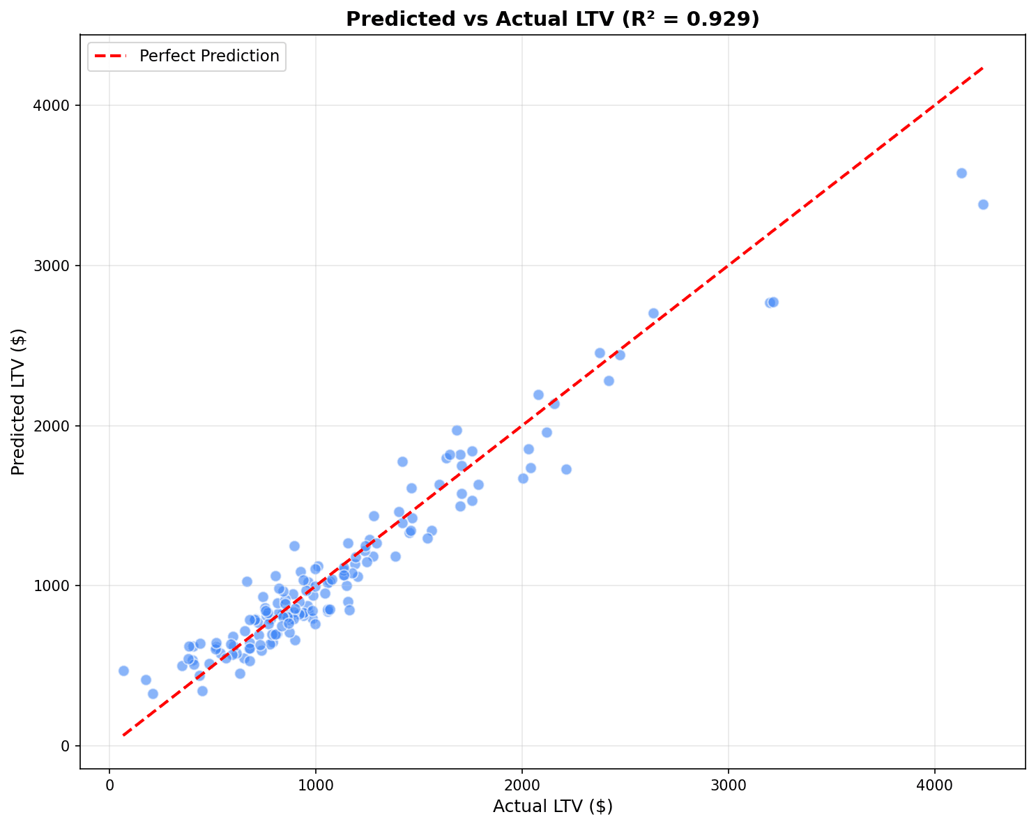
Points closer to the red diagonal line (perfect prediction) indicate a better model. R² closer to 1 means higher explanatory power.
Residual Analysis
# Residual analysis (based on best model)
residuals = y_test - y_pred_xgb

fig, axes = plt.subplots(1, 2, figsize=(12, 5))

# Residual distribution
axes[0].hist(residuals, bins=30, edgecolor='black', alpha=0.7)
axes[0].axvline(x=0, color='red', linestyle='--')
axes[0].set_xlabel('Residual ($)')
axes[0].set_ylabel('Frequency')
axes[0].set_title('Residual Distribution')

# Residual vs Predicted
axes[1].scatter(y_pred_xgb, residuals, alpha=0.5, s=20)
axes[1].axhline(y=0, color='red', linestyle='--')
axes[1].set_xlabel('Predicted CLV ($)')
axes[1].set_ylabel('Residual ($)')
axes[1].set_title('Residual vs Predicted')

plt.tight_layout()
plt.show()

# Residual statistics
print(f"Residual Mean: ${residuals.mean():,.2f}")
print(f"Residual Std: ${residuals.std():,.2f}")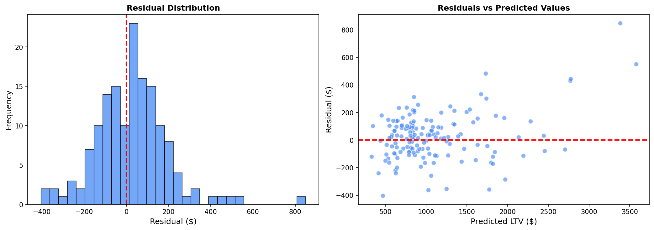
Characteristics of good model residuals:
- Residual distribution is normally distributed around 0
- No pattern in residual vs predicted, randomly dispersed
8. Cross-Validation
K-Fold Cross-Validation
from sklearn.model_selection import cross_val_score

# 5-Fold cross-validation
cv_scores = cross_val_score(
    xgb_model, X, y,
    cv=5,
    scoring='r2'
)

print("=== 5-Fold Cross-Validation ===")
print(f"R² Scores: {cv_scores.round(3)}")
print(f"Mean R²: {cv_scores.mean():.3f} (+/- {cv_scores.std():.3f})")=== 5-Fold Cross-Validation === R² Scores: [0.928 0.935 0.921 0.938 0.926] Mean R²: 0.930 (+/- 0.006)
Hyperparameter Tuning
from sklearn.model_selection import GridSearchCV

# Grid search
param_grid = {
    'n_estimators': [50, 100, 200],
    'max_depth': [4, 6, 8],
    'learning_rate': [0.05, 0.1, 0.2]
}

grid_search = GridSearchCV(
    XGBRegressor(random_state=42),
    param_grid,
    cv=3,
    scoring='r2',
    n_jobs=-1
)
grid_search.fit(X_train, y_train)

print("Best Parameters:", grid_search.best_params_)
print(f"Best R²: {grid_search.best_score_:.3f}")Best Parameters: {'learning_rate': 0.1, 'max_depth': 6, 'n_estimators': 100}
Best R²: 0.928Quiz 1: Evaluation Metric Selection
Problem
In a sales forecast model, which evaluation metric should you prioritize when:
- Prediction error needs to be interpretable in actual dollar amounts
- Overall error matters more than large individual errors
View Answer
Choose MAE (Mean Absolute Error).
Reasons:
- Interpretability: MAE can be intuitively interpreted as “on average, off by $X”
- Outlier robustness: Less sensitive to large errors
- Business meaning: Average error is important for budget planning
When to choose RMSE:
- When large prediction errors are particularly critical
- Example: Inventory excess/shortage causes significant costs
Quiz 2: R² Interpretation
Problem
A CLV prediction model has an R² of 0.65. How should you interpret this result?
View Answer
Interpretation:
- The model explains 65% of CLV variation
- 35% is explained by factors not included in the model
Business perspective:
- 0.65 is a practically acceptable level
- Perfect prediction (R²=1) is realistically impossible
- Sufficient for marketing budget allocation
Improvement directions:
- Add features (web behavior, customer demographics)
- Remove outliers
- Try non-linear models (XGBoost)
- Adjust time windows
Summary
Regression Model Selection Guide
| Situation | Recommended Model |
|---|---|
| Interpretation needed, linear relationship | Linear Regression |
| Multicollinearity issues | Ridge |
| Feature selection needed | Lasso |
| Non-linear relationships, large data | XGBoost |
Evaluation Metric Selection Guide
| Situation | Recommended Metric |
|---|---|
| Many outliers | MAE |
| Penalty for large errors | RMSE |
| Model explanatory power | R² |
| Scale-independent comparison | MAPE |
Next Steps
You’ve mastered regression prediction! Next, learn sales/demand forecasting using Prophet in Time Series Forecasting.