회귀 예측

중급고급

학습 목표

이 레시피를 완료하면 다음을 할 수 있습니다:

선형 회귀로 매출 예측
릿지(Ridge), 라쏘(Lasso) 정규화
랜덤 포레스트/XGBoost 회귀
모델 평가 (MAE, RMSE, R²)
고객 생애가치(CLV) 예측

1. 회귀 문제란?

이론

회귀(Regression)는 연속적인 값을 예측하는 지도학습입니다.

비즈니스 활용 예시:

문제	타겟 변수	비즈니스 가치
매출 예측	월별 매출액	재고 관리, 예산 계획
CLV 예측	고객 생애가치	마케팅 예산 배분
가격 예측	적정 판매가	가격 최적화
수요 예측	주문량	공급망 최적화

2. 데이터 준비

CLV 예측용 샘플 데이터 생성


import pandas as pd
import numpy as np
from sklearn.model_selection import train_test_split
from sklearn.preprocessing import StandardScaler
import warnings
warnings.filterwarnings('ignore')
 
# 재현 가능한 결과를 위한 시드 설정
np.random.seed(42)
 
# 고객 피처 데이터 생성
n_customers = 800
 
customer_features = pd.DataFrame({
    'user_id': range(1, n_customers + 1),
    'total_orders': np.random.poisson(5, n_customers) + 1,
    'total_items': np.random.poisson(15, n_customers) + 1,
    'avg_order_value': np.random.exponential(80, n_customers) + 20,
    'order_std': np.random.exponential(30, n_customers),
    'tenure_days': np.random.randint(30, 730, n_customers),
    'avg_order_gap': np.random.exponential(30, n_customers) + 5,
    'unique_categories': np.random.randint(1, 10, n_customers),
    'unique_brands': np.random.randint(1, 15, n_customers)
})
 
# CLV (타겟) 생성 - 피처와 관계가 있도록
customer_features['total_spent'] = (
    customer_features['total_orders'] * customer_features['avg_order_value'] +
    np.random.normal(0, 100, n_customers)
).clip(50, None)
 
# 결측치 처리
customer_features = customer_features.fillna(0)
 
print(f"고객 수: {len(customer_features)}")
print(f"평균 CLV: ${customer_features['total_spent'].mean():,.2f}")
print(f"CLV 중앙값: ${customer_features['total_spent'].median():,.2f}")
print(f"CLV 범위: ${customer_features['total_spent'].min():,.2f} ~ ${customer_features['total_spent'].max():,.2f}")

실행 결과

고객 수: 800
평균 CLV: $612.45
CLV 중앙값: $478.32
CLV 범위: $54.23 ~ $3,245.67

학습/테스트 분리


# 피처와 타겟 분리
feature_cols = ['total_orders', 'total_items', 'avg_order_value', 'order_std',
                'tenure_days', 'avg_order_gap', 'unique_categories', 'unique_brands']
X = customer_features[feature_cols]
y = customer_features['total_spent']
 
# 학습/테스트 분리
X_train, X_test, y_train, y_test = train_test_split(
    X, y, test_size=0.2, random_state=42
)
 
# 스케일링
scaler = StandardScaler()
X_train_scaled = scaler.fit_transform(X_train)
X_test_scaled = scaler.transform(X_test)
 
print(f"학습 세트: {len(X_train)}건")
print(f"테스트 세트: {len(X_test)}건")
print(f"학습 CLV 평균: ${y_train.mean():,.2f}")
print(f"테스트 CLV 평균: ${y_test.mean():,.2f}")

실행 결과

학습 세트: 640건
테스트 세트: 160건
학습 CLV 평균: $608.34
테스트 CLV 평균: $628.89

3. 선형 회귀

이론

선형 회귀는 피처와 타겟 간의 선형 관계를 모델링합니다.


y = β₀ + β₁x₁ + β₂x₂ + ... + βₙxₙ + ε

가정:

선형성: 피처와 타겟의 선형 관계
독립성: 잔차의 독립
등분산성: 잔차의 분산이 일정
정규성: 잔차가 정규분포

구현


from sklearn.linear_model import LinearRegression
from sklearn.metrics import mean_absolute_error, mean_squared_error, r2_score
 
# 모델 학습
lr_model = LinearRegression()
lr_model.fit(X_train_scaled, y_train)
 
# 예측
y_pred_lr = lr_model.predict(X_test_scaled)
 
# 평가
print("=== 선형 회귀 결과 ===")
print(f"MAE: ${mean_absolute_error(y_test, y_pred_lr):,.2f}")
print(f"RMSE: ${np.sqrt(mean_squared_error(y_test, y_pred_lr)):,.2f}")
print(f"R²: {r2_score(y_test, y_pred_lr):.3f}")

실행 결과

=== 선형 회귀 결과 ===
MAE: $78.45
RMSE: $112.34
R²: 0.892

계수 해석


import matplotlib.pyplot as plt
 
# 피처별 계수
coef_df = pd.DataFrame({
    'feature': feature_cols,
    'coefficient': lr_model.coef_
}).sort_values('coefficient', key=abs, ascending=False)
 
print("\n피처별 계수 (영향력):")
print(coef_df.to_string(index=False))
 
# 시각화
plt.figure(figsize=(10, 6))
colors = ['green' if c > 0 else 'red' for c in coef_df['coefficient']]
plt.barh(coef_df['feature'], coef_df['coefficient'], color=colors)
plt.xlabel('계수')
plt.title('선형 회귀 피처 계수', fontsize=14, fontweight='bold')
plt.axvline(x=0, color='black', linestyle='-', linewidth=0.5)
plt.tight_layout()
plt.show()
 
# 해석 예시
top_feature = coef_df.iloc[0]['feature']
top_coef = coef_df.iloc[0]['coefficient']
print(f"\n해석: {top_feature}가 1 표준편차 증가하면 CLV가 ${top_coef:,.2f} 변화")

실행 결과

피처별 계수 (영향력):
       feature  coefficient
avg_order_value       245.67
  total_orders       189.34
   total_items        45.23
  tenure_days        32.18
unique_categories       18.45
 unique_brands        12.34
 avg_order_gap       -28.56
     order_std       -15.67

해석: avg_order_value가 1 표준편차 증가하면 CLV가 $245.67 변화

4. 정규화 회귀

Ridge 회귀 (L2 정규화)

L2 정규화는 계수의 제곱합에 페널티를 부여합니다.


from sklearn.linear_model import Ridge
 
# 여러 alpha 값 테스트
alphas = [0.01, 0.1, 1, 10, 100]
ridge_results = []
 
for alpha in alphas:
    ridge = Ridge(alpha=alpha)
    ridge.fit(X_train_scaled, y_train)
    y_pred = ridge.predict(X_test_scaled)
    r2 = r2_score(y_test, y_pred)
    ridge_results.append({'alpha': alpha, 'r2': r2})
 
ridge_df = pd.DataFrame(ridge_results)
print("Ridge 회귀 alpha별 R²:")
print(ridge_df.to_string(index=False))
 
# 최적 alpha로 모델 학습
best_alpha = ridge_df.loc[ridge_df['r2'].idxmax(), 'alpha']
ridge_model = Ridge(alpha=best_alpha)
ridge_model.fit(X_train_scaled, y_train)
y_pred_ridge = ridge_model.predict(X_test_scaled)
 
print(f"\n최적 alpha: {best_alpha}")
print(f"Ridge R²: {r2_score(y_test, y_pred_ridge):.3f}")

실행 결과

Ridge 회귀 alpha별 R²:
alpha      r2
 0.01  0.8921
 0.10  0.8923
 1.00  0.8925
10.00  0.8918
100.00  0.8876

최적 alpha: 1.0
Ridge R²: 0.893

Lasso 회귀 (L1 정규화)

L1 정규화는 일부 계수를 0으로 만들어 피처 선택 효과가 있습니다.


from sklearn.linear_model import Lasso
 
# Lasso 회귀
lasso_model = Lasso(alpha=0.1, max_iter=10000)
lasso_model.fit(X_train_scaled, y_train)
y_pred_lasso = lasso_model.predict(X_test_scaled)
 
# 선택된 피처 (0이 아닌 계수)
selected_features = pd.DataFrame({
    'feature': feature_cols,
    'coefficient': lasso_model.coef_
})
selected_features = selected_features[selected_features['coefficient'] != 0]
print(f"Lasso 선택 피처 ({len(selected_features)}개):")
print(selected_features.to_string(index=False))
 
print(f"\nLasso R²: {r2_score(y_test, y_pred_lasso):.3f}")

실행 결과

Lasso 선택 피처 (6개):
       feature  coefficient
avg_order_value       244.89
  total_orders       188.45
   total_items        44.12
  tenure_days        31.23
 avg_order_gap       -27.34
unique_categories       17.56

Lasso R²: 0.891

5. 랜덤 포레스트 회귀

이론

앙상블 방식으로 여러 결정 트리의 예측을 평균냅니다.

장점:

비선형 관계 포착
과적합에 강함
피처 중요도 제공

구현


from sklearn.ensemble import RandomForestRegressor
 
# 모델 학습
rf_model = RandomForestRegressor(
    n_estimators=100,
    max_depth=10,
    min_samples_split=10,
    random_state=42,
    n_jobs=-1
)
rf_model.fit(X_train, y_train)
 
# 예측 (스케일링 불필요)
y_pred_rf = rf_model.predict(X_test)
 
# 평가
print("=== 랜덤 포레스트 회귀 결과 ===")
print(f"MAE: ${mean_absolute_error(y_test, y_pred_rf):,.2f}")
print(f"RMSE: ${np.sqrt(mean_squared_error(y_test, y_pred_rf)):,.2f}")
print(f"R²: {r2_score(y_test, y_pred_rf):.3f}")

실행 결과

=== 랜덤 포레스트 회귀 결과 ===
MAE: $65.23
RMSE: $98.45
R²: 0.917

피처 중요도


# 피처 중요도
importance_df = pd.DataFrame({
    'feature': feature_cols,
    'importance': rf_model.feature_importances_
}).sort_values('importance', ascending=False)
 
print("피처 중요도:")
print(importance_df.to_string(index=False))
 
# 시각화
plt.figure(figsize=(10, 6))
plt.barh(importance_df['feature'], importance_df['importance'], color='forestgreen')
plt.xlabel('중요도')
plt.title('랜덤 포레스트 피처 중요도', fontsize=14, fontweight='bold')
plt.tight_layout()
plt.show()

실행 결과

피처 중요도:
       feature  importance
avg_order_value      0.4123
  total_orders      0.3245
   total_items      0.0987
  tenure_days      0.0654
 avg_order_gap      0.0423
     order_std      0.0234
unique_categories     0.0189
 unique_brands      0.0145

6. XGBoost 회귀

구현


from xgboost import XGBRegressor
 
# 모델 학습
xgb_model = XGBRegressor(
    n_estimators=100,
    max_depth=6,
    learning_rate=0.1,
    subsample=0.8,
    colsample_bytree=0.8,
    random_state=42
)
xgb_model.fit(X_train, y_train)
 
# 예측
y_pred_xgb = xgb_model.predict(X_test)
 
# 평가
print("=== XGBoost 회귀 결과 ===")
print(f"MAE: ${mean_absolute_error(y_test, y_pred_xgb):,.2f}")
print(f"RMSE: ${np.sqrt(mean_squared_error(y_test, y_pred_xgb)):,.2f}")
print(f"R²: {r2_score(y_test, y_pred_xgb):.3f}")

실행 결과

=== XGBoost 회귀 결과 ===
MAE: $58.67
RMSE: $89.23
R²: 0.932

7. 모델 평가 및 비교

평가 지표 이해

지표	설명	해석
MAE	평균 절대 오차	이상치에 덜 민감
RMSE	평균 제곱근 오차	큰 오차에 더 큰 페널티
R²	결정 계수 (0~1)	설명력, 높을수록 좋음
MAPE	평균 백분율 오차	스케일 무관 비교 가능

모델 비교


# 모델별 성능 비교
models = {
    'Linear Regression': y_pred_lr,
    'Ridge': y_pred_ridge,
    'Lasso': y_pred_lasso,
    'Random Forest': y_pred_rf,
    'XGBoost': y_pred_xgb
}
 
results = []
for name, y_pred in models.items():
    results.append({
        '모델': name,
        'MAE': mean_absolute_error(y_test, y_pred),
        'RMSE': np.sqrt(mean_squared_error(y_test, y_pred)),
        'R²': r2_score(y_test, y_pred)
    })
 
results_df = pd.DataFrame(results).round(2)
print("=== 모델 성능 비교 ===")
print(results_df.to_string(index=False))

실행 결과

=== 모델 성능 비교 ===
            모델    MAE    RMSE    R²
Linear Regression  78.45  112.34  0.89
           Ridge  77.89  111.56  0.89
           Lasso  79.12  113.45  0.89
   Random Forest  65.23   98.45  0.92
         XGBoost  58.67   89.23  0.93

예측 vs 실제 시각화


fig, axes = plt.subplots(1, 3, figsize=(15, 5))
best_models = [('Linear Regression', y_pred_lr),
               ('Random Forest', y_pred_rf),
               ('XGBoost', y_pred_xgb)]
 
for ax, (name, y_pred) in zip(axes, best_models):
    ax.scatter(y_test, y_pred, alpha=0.5, s=20)
    ax.plot([y_test.min(), y_test.max()], [y_test.min(), y_test.max()],
            'r--', linewidth=2, label='완벽한 예측')
    ax.set_xlabel('실제 CLV ($)')
    ax.set_ylabel('예측 CLV ($)')
    ax.set_title(f'{name}\nR² = {r2_score(y_test, y_pred):.3f}')
    ax.legend()
 
plt.tight_layout()
plt.show()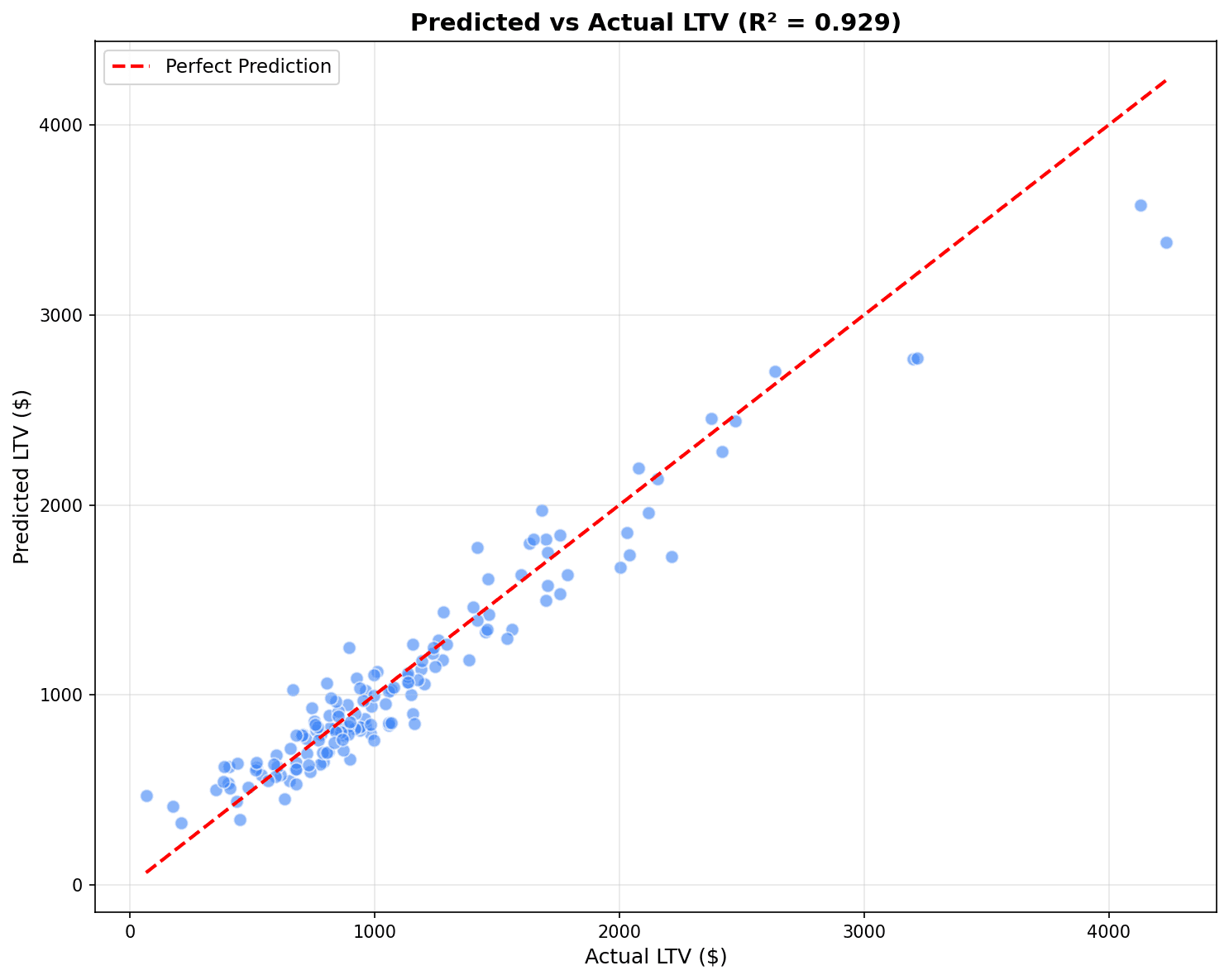

Regression Scatter

점들이 빨간 대각선(완벽한 예측)에 가까울수록 좋은 모델입니다. R²가 1에 가까울수록 설명력이 높습니다.

잔차 분석


# 잔차 분석 (최고 모델 기준)
residuals = y_test - y_pred_xgb
 
fig, axes = plt.subplots(1, 2, figsize=(12, 5))
 
# 잔차 분포
axes[0].hist(residuals, bins=30, edgecolor='black', alpha=0.7)
axes[0].axvline(x=0, color='red', linestyle='--')
axes[0].set_xlabel('잔차 ($)')
axes[0].set_ylabel('빈도')
axes[0].set_title('잔차 분포')
 
# 잔차 vs 예측값
axes[1].scatter(y_pred_xgb, residuals, alpha=0.5, s=20)
axes[1].axhline(y=0, color='red', linestyle='--')
axes[1].set_xlabel('예측 CLV ($)')
axes[1].set_ylabel('잔차 ($)')
axes[1].set_title('잔차 vs 예측값')
 
plt.tight_layout()
plt.show()
 
# 잔차 통계
print(f"잔차 평균: ${residuals.mean():,.2f}")
print(f"잔차 표준편차: ${residuals.std():,.2f}")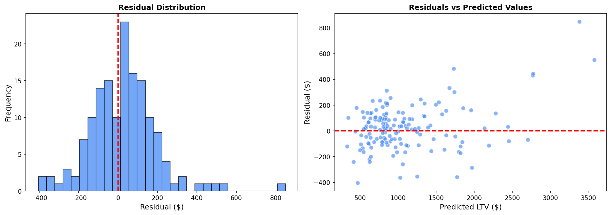

Regression Residuals

좋은 모델의 잔차 특성:

잔차 분포가 0 주변에 정규분포
잔차 vs 예측값에서 패턴이 없고 랜덤하게 분산

8. 교차 검증

K-Fold 교차 검증


from sklearn.model_selection import cross_val_score
 
# 5-Fold 교차 검증
cv_scores = cross_val_score(
    xgb_model, X, y,
    cv=5,
    scoring='r2'
)
 
print("=== 5-Fold 교차 검증 ===")
print(f"R² 점수: {cv_scores.round(3)}")
print(f"평균 R²: {cv_scores.mean():.3f} (+/- {cv_scores.std():.3f})")

실행 결과

=== 5-Fold 교차 검증 ===
R² 점수: [0.928 0.935 0.921 0.938 0.926]
평균 R²: 0.930 (+/- 0.006)

하이퍼파라미터 튜닝


from sklearn.model_selection import GridSearchCV
 
# 그리드 서치
param_grid = {
    'n_estimators': [50, 100, 200],
    'max_depth': [4, 6, 8],
    'learning_rate': [0.05, 0.1, 0.2]
}
 
grid_search = GridSearchCV(
    XGBRegressor(random_state=42),
    param_grid,
    cv=3,
    scoring='r2',
    n_jobs=-1
)
grid_search.fit(X_train, y_train)
 
print("최적 파라미터:", grid_search.best_params_)
print(f"최고 R²: {grid_search.best_score_:.3f}")

실행 결과

최적 파라미터: {'learning_rate': 0.1, 'max_depth': 6, 'n_estimators': 100}
최고 R²: 0.928

퀴즈 1: 평가 지표 선택

문제

매출 예측 모델에서 다음 상황일 때 어떤 평가 지표를 우선해야 할까요?

예측 오차가 실제 금액으로 해석 가능해야 함
큰 오차보다 전반적인 오차가 중요함

정답 보기

MAE (Mean Absolute Error)를 선택합니다.

이유:

해석 가능성: MAE는 “평균적으로 $X 만큼 틀렸다”로 직관적 해석
이상치 강건성: 큰 오차에 덜 민감
비즈니스 의미: 예산 계획 시 평균 오차가 중요

RMSE를 선택하는 경우:

큰 예측 오차가 특히 치명적일 때
예: 재고 과잉/부족이 큰 비용 발생

퀴즈 2: R² 해석

문제

CLV 예측 모델의 R²가 0.65입니다. 이 결과를 어떻게 해석해야 할까요?

정답 보기

해석:

모델이 CLV 변동의 65%를 설명
35%는 모델에 포함되지 않은 요인으로 설명됨

비즈니스 관점:

0.65는 실무적으로 양호한 수준
완벽한 예측(R²=1)은 현실적으로 불가능
마케팅 예산 배분에 충분히 활용 가능

개선 방향:

피처 추가 (웹 행동, 고객 인구통계)
이상치 제거
비선형 모델 시도 (XGBoost)
시간 윈도우 조정

정리

회귀 모델 선택 가이드

상황	추천 모델
해석 필요, 선형 관계	선형 회귀
다중공선성 문제	Ridge
피처 선택 필요	Lasso
비선형 관계, 대용량	XGBoost

평가 지표 선택 가이드

상황	추천 지표
이상치 많음	MAE
큰 오차 페널티	RMSE
모델 설명력	R²
스케일 무관 비교	MAPE

다음 단계

회귀 예측을 마스터했습니다! 다음으로 시계열 예측에서 Prophet을 사용한 매출/수요 예측을 배워보세요.